Prepare sorted variants in vcf format. The INFO field in each entry includes a sample ID in SAMPLE={sample_id} format.
#CHROM  POS ID  REF ALT QUAL    FILTER  INFO
chr1    3747728 .        T       C       .       .       SAMPLE=11000.p1
chr1    38338861        .       C       A       .       .       SAMPLE=11000.p1
chr1    117942118       .      T       G       .       .       SAMPLE=11000.p1
Sample information
Prepare the sample information in a text file, such as in txt or tsv format. The file must be tab separated. It also must contain three columns, SAMPLE and PHENOTYPE. A value in the PHENOTYPE muse be case or ctrl.
The values in the SAMPLE column are matched to the sample IDs of variants in the input vcf file.
SAMPLE
PHENOTYPE
11000.p1
case
11000.s1
ctrl
11002.p1
case
11002.s1
ctrl
Adjustment factors
Adjustment factors are required if the users want to adjust the number of variants for each sample in CWAS-Plus2. The file must be tab separated and must contain two columns, SAMPLE and AdjustFactor. A value in the AdjustFactor must be a float.
The values in the SAMPLE column must be matched to the sample IDs of variants in the input vcf file.
cd $HOME
git clone https://github.com/joonan-lab/cwas-input-example.git
Annotation dataset
CWAS-Plus2 requires annotation dataset to annotate and categorize variants. Users can customize their own annotation dataset based on ther interest.
For example run, annotation datasets for investigating autism spectrum disorder are available at joonan-lab/cwas-dataset.
cd $HOME
git clone https://github.com/joonan-lab/cwas-dataset.git
Required installations
Conda: CWAS-Plus2 is installed in a conda environment, so conda should be installed.
VEP: For variant annotation, VEP should be installed. Please refer to the reference.
CWAS-Plus2 requires a working directory for efficiency. Users can create the working directory through command below.
cwasstart
By default, the command creates a working directory (.cwas) in the home directory. However, if users want to set the working directory manually, they can use -w option to specify the path of the desired working directory.
cwasstart-w/path/to/the/working/directory
The command cwasstart, also creates a configuration file inside the working directory. If there is a pre-installed VEP, the path of the VEP in the configuration file will be automatically set.
Inside the CWAS working directory, there is a configuration file (configuration.txt). This file is needed for retrieving the path of specific files needed for CWAS-Plus2 run.
With pre-installed VEP, the configuration file looks like below.
ANNOTATION_DATA_DIR: This is the path of the directory, which contains annotation datasets, such as bed files.
GENE_MATRIX: This is the file name of the gene matrix, which is a text file. The first column should be gene ID, and the second column should be gene name. The other columns will represent each gene list and show whether each row (=gene) are matched to the gene list or not by a binary code (0, 1). 1 if the gene is matched to a gene list, 0 if not.
ANNOTATION_KEY_CONFIG: This is the file name of the annotation key file, which is a yaml file. This file contains the name of the annotation datasets inside the annotation dataset directory and the key names that will be used to represent the dataset. All details should be written in yaml syntax. Also, to split the category group to functional score and functional annotation, the users should type each annotation dataset under the matched group dictionary. Below is an example of this file. The format should be (name): (key) with a uniform indentation for each row. Be aware that the name of the annotations should not contain ‘_’. As domains will combined with ‘_’ as a delimiter, using ‘_’ in the annotation name will cause errors.
VEP: This is the path of VEP. If there is a pre-installed VEP, this line would be written in advance when the users typed the command cwasstart.
VEP_CACHE_DIR: This is the path of the directory, which contains cache files and overall resources for VEP.
VEP_CONSERVATION_FILE: This is the path of the conservation file (loftee.sql), which will be used for variant classification.
VEP_LOFTEE: This is the file name of the directory of loftee plugin, which will be used for variant classification.
VEP_HUMAN_ANCESTOR_FA: This is the file name of the human ancestor fasta file, which will be used for variant classification.
VEP_GERP_BIGWIG: This is the file name of the GERP bigwig file, which will be used for variant classification.
VEP_MIS_DB: This is the file name of the database in vcf format. This will be used for variant classification. Users can manually prepare this file to classify damaging missense variants.
VEP_MIS_INFO_KEY: The name of the score in the missense classification database. It must be present in the INFO field of the database. The score must be specified by this name in the field. For example, if the user is using MPC score in the database, the database will look like below.
#CHROM
POS
ID
REF
ALT
QUAL
FILTER
INFO
chr1
69094
.
G
A
.
.
MPC=2.73403
chr1
69094
.
G
C
.
.
MPC=2.29136
chr1
69094
.
G
T
.
.
MPC=2.29136
chr1
69095
.
T
A
.
.
MPC=4.31666
VEP_MIS_THRES: The cutoff that will be used for the missense classification. The missense variants scoring equal to or above VEP_MIS_THRES will be classified as damaging missense mutations.
By default, CWAS-Plus2 provides all of the data above (except for VEP) and configuration file (configuration.txt) through joonan-lab/cwas-dataset. Please note that the provided data serves as default examples, which users can customize to their specific needs.
To use VEP, users need cache file matching to the VEP version. The cache file can be found here. Please download the file in the VEP_CACHE_DIR.
To download required resources and annotation datasets in GRCh38 version in one step, run the command below. It will create directory ($HOME/.vep) and download resources in the directory. By default, the resources are in the child directory of the home directory.
cd $HOME
git clone https://github.com/joonan-lab/cwas-dataset.git
cd cwas-dataset
git lfs pull
tar -zxvf functional_annotations.tar.gz # Decompress bed files
mv functional_annotations/* . # Move bed files to the parent directory
sh download_vep_resources.sh
mv $HOME/cwas-dataset/MPC_hg38.vcf.bgz* $HOME/.vep/ # Move MPC files to VEP_CACHE_DIR
The downloading time could be close to three hours, depending on the speed of the network.
The descriptions of the files in the cwas-dataset are as below.
annotation_keys.yaml: List of annotation datasets with the exact file names and short names used for CWAS-Plus2 annotation.
gene_matrix.txt: List of genes with their functional annotations.
download_vep_resources.sh: Code to download VEP resources.
configuration.txt: Configuration file for CWAS-Plus2 specifying VEP path and required resources.
functional_annotations.tar.gz: BED files for annotating variants. After decompressing, please move the files within the directory to the parent directory “cwas-dataset.”
MPC_hg38.vcf.bgz: Database for annotation damaging missense variants. For further information, please refer to the provided reference.
BED files for vertebrate conservation scores
PhyloP46way and PhastCons46Way
Due to the large file sizes, we provide an alternative download link for the original files.
When preparing the ANNOTATION_KEY_CONFIG yaml file, please avoid using underscores (‘_’) in the annotation name. Underscores are used for distinguishing different domains within a single category.
For example, check below.
functional_score:
  bed1.bed.gz: annot1
  bed2.bed.gz: annot2
functional_annotation:
  bed3.bed.gz: annot_3 # Do not use underscores like this. Users can use 'annot3' instead.
  bed4.bed.gz: annot4
After preparing all resources, fill in the configuration.txt file with specific paths to the file.
For example run, you can copy the configuration.txt in the cwas-dataset to the CWAS-Plus2 working directory.
Before running configuration, please check things below.
Check the VEP path and modify VEP with the exact path.
Check the path to ANNOTATION_DATA_DIR and VEP_CACHE_DIR.
Move MPC_hg38.vcf.bgz from cwas-dataset to VEP_CACHE_DIR.
All bed files should be indexed using tabix.
The BED files, GENE_MATRIX, and ANNOTATION_KEY_CONFIGmust be inside ANNOTATION_DATA_DIR.
The VEP_CONSERVATION_FILE, VEP_LOFTEE, VEP_HUMAN_ANCESTOR_FA, VEP_GERP_BIGWIG, VEP_GERP_BIGWIG, and VEP_MIS_DBmust be inside VEP_CACHE_DIR.
For GENE_MATRIX, ANNOTATION_KEY_CONFIG, VEP_MIS_DB, VEP_CONSERVATION_FILE, VEP_LOFTEE, VEP_HUMAN_ANCESTOR_FA, VEP_GERP_BIGWIG and VEP_GERP_BIGWIGmust be only file names, not the absolute path. For instance, if VEP_CACHE_DIR is /home/user/.vep and the file name of VEP_GERP_BIGWIG is file.bw, VEP_GERP_BIGWIG should only be specified as file.bw, excluding the complete path.
After filling the configuration file, cwasconfiguration command will create symlinks of annotation datasets into the working directory.
The command will also add environment variables for CWAS-Plus2 in the .cwas_env file in the home directory. To force configuration (overwrite previous configurations), use -f option.
Gather and merge functional annotations and scores into a single bed file. The annotation datasets in the ANNOTATION_DATA_DIR will be merged to a single bed file in the working directory.
The parameters of the command are as below:
p: The number of processors.
cwaspreparation-p8
After running the command, merged BED file and its index will be generated in your CWAS workspace.
Annotate the input VCF file with VEP and bed custom annotation algorithm.
When using more than one worker processes, CWAS-Plus2 automatically bgzip and indexes non-gzipped input files for efficient multiprocessing.
Output files are stored in the designated output directory (-o_dir) or, by default, in the working directory ($CWAS_WORKSPACE).
The parameters of the command are as below:
-v, –vcf_file: Path to the input vcf file. This file could be bgzipped or not.
-p, –num_proc: Number of worker processes that will be used for the annotation process. By default, 1.
-o_dir, –output_directory: Path to the directory where the output files will be saved. By default, outputs will be saved at $CWAS_WORKSPACE.
–docker-mode: Run VEP using Docker (ensemblorg/ensembl-vep) instead of a local binary. With this option, a local VEP installation is not required. By default, False.
–vep-version: VEP version for Docker image tag (e.g. 115.0). Only used with --docker-mode. If omitted, uses latest.
cwasannotation-vINPUT.vcf-o_dirOUTPUT_DIR-p8
The specific descriptions of the output files are as below. Each output file containing a specific pattern (i.e., .vep.vcf.gz, .vep.vcf.gz.tbi, .annotated.vcf) in the file name as below will be found in the output directory.
OUTPUT.vep.vcf.gz: VEP annotated output file. This file is an intermediate output that has not been annotated with bed annotation files yet.
OUTPUT.vep.vcf.gz.tbi: Index file of the OUTPUT.vep.vcf.gz.
OUTPUT.annotated.vcf: The final output file. This file will be used as an input for categorization process.
The de_novo_variants.annotated.vcf.gz looks like below. The number following ANNOT= in the INFO field indicates specific annotations associated with the variant, which will be decoded into binary code representing the relevant annotations.
##fileformat=VCFv4.1
##VEP="v105" time="2023-07-13 11:51:32" cache="/home/cwas_testing/.vep/homo_sapiens/105_GRCh38" ensembl-funcgen=105.660df8f ensembl-io=105.2a0a40c ensembl-variation=105.ac8178e ensembl=105.525fbcb 1000genomes="phase3" COSMIC="92" ClinVar="202106" ESP="V2-SSA137" HGMD-PUBLIC="20204" assembly="GRCh38.p13" dbSNP="154" gencode="GENCODE 39" genebuild="2014-07" gnomAD="r2.1.1" polyphen="2.2.2" regbuild="1.0" sift="sift5.2.2"
##INFO=<ID=CSQ,Number=.,Type=String,Description="Consequence annotations from Ensembl VEP. Format: Allele|Consequence|IMPACT|SYMBOL|Gene|Feature_type|Feature|BIOTYPE|EXON|INTRON|HGVSc|HGVSp|cDNA_position|CDS_position|Protein_position|Amino_acids|Codons|Existing_variation|DISTANCE|STRAND|FLAGS|SYMBOL_SOURCE|HGNC_ID|SOURCE|NEAREST|LoF|LoF_filter|LoF_flags|LoF_info|MisDb|MisDb_MPC">
##LoF=Loss-of-function annotation (HC = High Confidence; LC = Low Confidence)
##LoF_filter=Reason for LoF not being HC
##LoF_flags=Possible warning flags for LoF
##LoF_info=Info used for LoF annotation
##INFO=<ID=MisDb,Number=.,Type=String,Description="/home/cwas_testing/cwas-dataset/MPC_hg38.vcf.bgz (exact)">
##INFO=<ID=MisDb_MPC,Number=.,Type=String,Description="MPC field from /home/cwas_testing/cwas-dataset/MPC_hg38.vcf.bgz">
##INFO=<ID=ANNOT,Key=phastCons46way|phyloP46way|ChmE1|ChmE10|ChmE11|ChmE12|ChmE13|ChmE14|ChmE15|ChmE2|ChmE3|ChmE4|ChmE5|ChmE6|ChmE7|ChmE8|ChmE9|EpiDNase|EpiH3K27ac|EpiH3K27me3|EpiH3K36me3|EpiH3K4me1|EpiH3K4me3|EpiH3K9ac|EpiH3K9me3|MidFetalH3K27ac|YaleH3K27acCBC|YaleH3K27acDFC|MidFetalATAC|EncodeDNase|EncodeTFBS|EnhancerVista|EnhancerFantom|HARs>
#CHROM      POS     ID      REF     ALT     QUAL    FILTER  INFO
chr1        822758  chr1:822758:C:T C       T       .       .       SAMPLE=11299.s1;CSQ=T|intron_variant&non_coding_transcript_variant|MODIFIER||ENSG00000230021|Transcript|ENST00000635509|processed_transcript||1/3||||||||||-1|||||SAMD11||||||;ANNOT=33313024
chr1        842732  chr1:842732:G:A G       A       .       .       SAMPLE=13373.p1;CSQ=A|non_coding_transcript_exon_variant|MODIFIER|LINC01128|ENSG00000228794|Transcript|ENST00000670780|lncRNA|3/8||||1807|||||||1||HGNC|HGNC:49377||SAMD11||||||;ANNOT=764418304
chr1        843980  chr1:843980:A:G A       G       .       .       SAMPLE=13807.s1;CSQ=G|non_coding_transcript_exon_variant|MODIFIER|LINC01128|ENSG00000228794|Transcript|ENST00000670780|lncRNA|3/8||||3055|||||||1||HGNC|HGNC:49377||SAMD11||||||;ANNOT=754716928
Categorize variants into groups based on the annotation datasets. A single category is a combination of five domains (i.e., variant type, gene biotype, gene list, functional annotation and functional score). Details are provided in the Overview of annotation datasets.
The input file is the final output file resulted from annotation process. To generate correlation matrices between categories, use the separate cwascorrelation step after categorization.
The parameters of the command are as below:
-i, –input_file: Path to the annotated VCF, resulted from annotation process. This file contains a specific pattern of .annotated.vcf in the file name. This file could be gzipped or not.
-o_dir, –output_directory: Path to the directory where the output files will be saved. By default, outputs will be saved at $CWAS_WORKSPACE.
-p, –num_proc: Number of worker processes that will be used for the categorization process. To prevent crashes caused by insufficient RAM when processing large input VCF files (e.g., over 10 million variants) using multiple cores, using small number of cores and monitoring the memory usage are recommended. By default, 1.
The specific descriptions of the output files are as below. The output file containing a specific pattern (i.e., .categorization_result.zarr) in the file name as below will be found in the output directory.
OUTPUT.categorization_result.zarr: The final output file containing the number of variants in each category across samples. This file will be used as input in the burden test process.
The de_novo_variants.categorization_result.zarr looks like below. The “SAMPLE” column refers to the sample ID. Each of the other columns corresponds to a specific category. The values in these columns represent the number of variants within each category, specifically for each sample.
Calculate the burden of each category by calculating the burden of each category by comparing the rate of variants per cases and the rate of variants per controls.
For burden measurement, the package uses relative risk (RR), which is calculated by comparing the number of variants per phenotype group (RR>1, case burden; RR<1, control burden). The burden test in CWAS-Plus2 contains two types of p-value computation methods, binomial test and permutation test, to find more accurate p statistics.
Binomial test
-i, –input_file: Path to the categorized zarr directory, resulted from categorization process.
-o_dir, –output_directory: Path to the directory where the output files will be saved. By default, outputs will be saved at $CWAS_WORKSPACE.
-s, –sample_info: Path to the txt file containing the sample information for each sample. This file must have three columns (SAMPLE, FAMILY, PHENOTYPE) with the exact name.
-a, –adjustment_factor: Path to the txt file containing the adjust factors for each sample. This is optional. With this option, CWAS-Plus2 multiplies the number of variants (or carriers, in -u option) with the adjust factor per sample.
-u, –use_n_carrier: Enables the sample-level analysis (use of the number of samples with variants in each category for burden test instead of the number of variants). With this option, CWAS-Plus2 counts the number of samples that carry at least one variant of each category.
-i, –input_file: Path to the categorized zarr directory, resulted from categorization process.
-o_dir, –output_directory: Path to the directory where the output files will be saved. By default, outputs will be saved at $CWAS_WORKSPACE.
-s, –sample_info: Path to the txt file containing the sample information for each sample. This file must have three columns (SAMPLE, FAMILY, PHENOTYPE) with the exact name.
-a, –adjustment_factor: Path to the txt file containing the adjust factors for each sample. This is optional. With this option, CWAS-Plus2 multiplies the number of variants (or carriers, in -u option) with the adjust factor per sample.
-n, –num_perm: Number of permutations for label-swapping. By default, 10000.
-p, –num_proc: Number of worker processes that will be used for the permutation process. By default, 1.
-b, –burden_shift: Generates an output file containing binomial p-values for each label-swapped permutation. By default, False.
-u, –use_n_carrier: Enables the sample-level analysis (use of the number of samples with variants in each category for burden test instead of the number of variants). With this option, CWAS-Plus2 counts the number of samples that carry at least one variant of each category.
The specific descriptions of the output files are as below. Each output file containing a specific pattern (i.e., .burden_test.txt, .permutation_test.txt.gz, .binom_pvals.parquet) in the file name as below will be found in the output directory.
OUTPUT.burden_test.txt: The final output file containing relative risk, two-sided binomial p-value and one-sided binomial p-value of each category.
OUTPUT.permutation_test.txt.gz: The final output file containing p-values calculated from permutations. This file will be used for DAWN analysis.
OUTPUT.binom_pvals.parquet: The matrix containing binomial p-values generated from each permutation (saved in Apache Parquet format). This file will be generated only with -b option given.
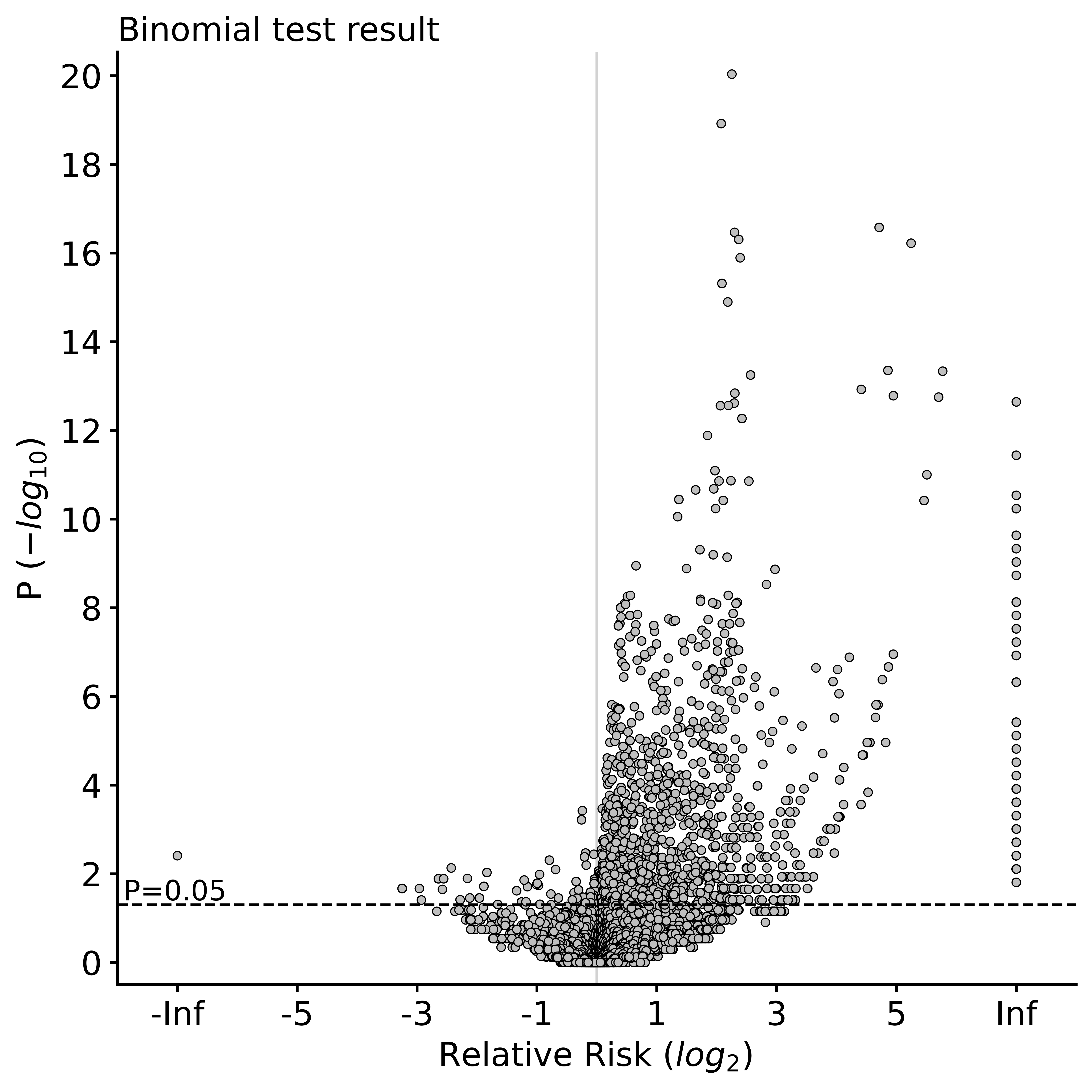
The de_novo_variants.burden_test.volcano_plot.pdf looks like below. Each dot in the plot is a category. The x axis refers to two-sided binomial p-values in -log10 format. The y axis refers to the relative risk in log2 format. The red dashed line represents a p-value threshold of 0.05.
The de_novo_variants.burden_test.txt looks like below. This output file contains the burden and significance of each category resulted from burden test.
variant_type: The variant type of the variants in the category.
gene_list: The name of the specific gene list to which the genes in the category belong.
conservation: The name of the specific functional score domain region to which the variants in the category belong.
gencode: The gene biotype (such as coding, noncoding, promoter, etc.) of the variants within the category.
region: The name of the specific region from functional region domain to which the variants in the category belong.
Case_DNV_Count: The number of variants in cases within the category.
Ctrl_DNV_Count: The number of variants in controls within the category.
Relative_Risk: The ratio of (# of variants in cases / # of cases) divided by (# of variants in controls / # of controls). If Relative_Risk is greater than 1, the category indicates a case burden. On the other hand, if Relative_Risk is less than 1, the category suggests a control burden.
P: Two-sided binomial p-value.
P_1side: One-sided binomial p-value with an alternative hypothesis of ‘greater’. This indicates that it measures the statistical significance of the expected proportion of the number of variants in cases being greater than the proportion of cases in the total samples.
Z_1side: Z-score calculated from the one-sided binomial p-value.
The de_novo_variants.category_counts.txt looks like below. This output file contains the number of variants in each category.
Raw_counts: The number of variants in the category. Not adjusted.
Adj_counts: The adjusted number of variants in the category.
The de_novo_variants.category_info.txt looks like below. This output file contains the additional information about the category that are useful to the users. Specifically, columns starting with is_ indicate the respective group to which each category belongs, based on the gene biotype domain.
For instance, categories that have 1 in is_coding colmn are coding categories.
variant_type: The variant type of the variants in the category.
gene_list: The name of the specific gene list to which the genes in the category belong.
conservation: The name of the specific functional score domain region to which the variants in the category belong.
gencode: The gene biotype (such as coding, noncoding, promoter, etc.) of the variants within the category.
region: The name of the specific region from functional region domain to which the variants in the category belong.
Case_DNV_Count: The number of variants in cases within the category.
Ctrl_DNV_Count: The number of variants in controls within the category.
Relative_Risk: The ratio of (# of variants in cases / # of cases) divided by (# of variants in controls / # of controls). If Relative_Risk is greater than 1, the category indicates a case burden. On the other hand, if Relative_Risk is less than 1, the category suggests a control burden.
P: Permutation p-value. Calculated by comparing the relative risks from permuted outputs and the observed relative risk.
The de_novo_variants.binom_pvals.parquet looks like below. This file is saved in Apache Parquet format and is used in the burden shift analysis. The Trial column refers to each permutation. Other columns indicate the p-values of each category. Positive p-values indicate categories enriched in cases and negative p-values indicate categories enriched in controls. This distinguishment is for the burden shift analysis (to count the number of significant categories in each phenotype).
For (1) calculating study-wide significance threshold and (2) generating DAWN analysis input, correlation values between every two CWAS categories are required.
In this step, users can generate two matrices, (1) a matrix that contains the number of variants (or samples, with –use_carrier option) that intersect between categories, (2) a matrix that contains correlation values between categories. The correlation matrix is computed from the intersected matrix (1). The users can choose one of the matrices for calculating the number of effective tests and DAWN analysis.
The parameters of the command are as below:
-i, –input_file: Path to the categorized zarr directory, resulted from categorization process.
-v, –annotated_vcf: Path to the annotated VCF, resulted from annotation process. Required for variant-level correlation matrix (–cm variant).
-o_dir, –output_directory: Path to the directory where the output files will be saved. By default, outputs will be saved at $CWAS_WORKSPACE.
-p, –num_proc: Number of worker processes that will be used for the categorization process. To prevent crashes caused by insufficient RAM when processing large input VCF files (e.g., over 10 million variants) using multiple cores, using small number of cores and monitoring the memory usage are recommended. By default, 1.
-cm, –corr_matrix: (Required) Generate a correlation matrix between every two categories. Available options are variant or sample.
variant: Use the intersected number of variants between two categories.
sample: Use the intersected number of samples between two categories.
-im, –intersection_matrix: Generate a matrix with intersected number of variants (or samples with variants) bewteen categories.
-c_info, –category_info: Path to a text file with category information (*.category_info.txt).
-d, –domain_list: Domain list to filter categories based on GENCODE domain. By default, all.
Calculating the correlation matrix takes about 139 minutes with eight cores.
The specific descriptions of the output files are as below. The utput file containing a specific pattern (i.e., .intersection_matrix.zarr, .correlation_matrix.zarr) in the file name as below will be found in the output directory.
OUTPUT.intersection_matrix.zarr: The matrix containing the number of intersected variants (or samples) between every two categories.
OUTPUT.correlation_matrix.zarr: The matrix containing the correlation values between every two categories. This file will be used for calculating the number of effective tests. This file will be used as an input for DAWN analysis.
From correlation matrix, compute eigen values and vectors. Based on these outputs, users can calculate the number of effective tests.
The outputs of this command can also be used for DAWN analysis. More detailed explanations are below the description of parameters.
The parameters of the command are as below:
-i, –input_file: Path to a matrix of correlation or intersected number of variants between two categories.
-if, –input_format: Specify the format of the input file. Available options are corr or inter. By default, corr will be used. Each format refers to the following:
corr: A matrix with correlation values between categories.
inter: A matrix with intersected number of variants (or samples) between categories.
-o_dir, –output_directory: Path to the directory where the output files will be saved. By default, outputs will be saved at $CWAS_WORKSPACE.
-n, –num_eig: Number of eigen values to use in calculating the number of effective tests. The maximum number is equivalent to the number of categories. By default, 10000.
-s, –sample_info: Path to the txt file containing the sample information for each sample. This file must have three columns (SAMPLE, FAMILY, PHENOTYPE) with the exact name. Required only when input format is set to inter or -thr is not given. By default, None.
-c_count, –cat_count: Path of the categories counts file from binomial burden test (*.category_counts.txt).
-t, –tag: Tag used for the name of the output files. By default, None.
-c_set, –category_set: Path to a text file containing categories for eigen decomposition. If not specified, all of the categories (surpassing the cutoff) will be used. This file must contain Category column with the name of categories to be used.
-ef, –eff_num_test: Calculate the effective number of tests. For calculation, the users should use all categories (with the number of variants/samples≥cutoff). By default, False.
-thr, –threshold: The number of variants (or samples) to filter categories. By default, None.
Find the number of effective tests
Only categories with a value (number of variants or samples) greater than or equal to cutoff are used. The cutoff is used to select informative significant tests with a sufficient number of variants (or samples).
With specified cutoff: Categories with a value (number of variants or samples) greater than or equal to specified cutoff are used.
Without specified cutoff: The cutoff is automatically calculated and applied to filter categories with a value (number of variants or samples) greater than or equal to cutoff. The cutoff represents the minimum number of variants (or samples) required for a one-sided binomial test with p<0.05, assuming the null hypothesis is a Binomial(m, No. cases/No. total samples) distribution with 1 mutation in controls and m-1 mutations in cases.
Use the identical cutoff for the number of variants (or samples) as in 1.Findthenumberofeffectivetests, while focusing only on specific categories relevant to the users’ domains of interest. For example, users can exclusively use intergenic categories. Aditionally, when generating DAWN analysis inputs, omit the-efargument, as the number of effective tests calculated for this subset of categories of interest will not be used elsewhere.
The specific descriptions of the output files are as below. Each output file containing a specific pattern (i.e., .neg_lap.*.zarr, .eig_vals.*.zarr, .eig_vecs.*.zarr) in the file name as below will be found in the output directory. If users set tag, the tag will be inserted in the file name like this: OUTPUT.eig_vecs.tag.zarr.
OUTPUT.neg_lap.zarr: The negative laplacian matrix. This file is an intermediate output during eigen decomposition.
OUTPUT.eig_vals.zarr: The matrix containing eigen values. This file will be used to calculate the number of effective tests.
OUTPUT.eig_vecs.zarr: The matrix containing eigen vectors. This file will be used as an input for DAWN analysis.
In addition, the number of effective tests will be printed as below when -ef option is given. The number will also be written in .cwas_env as environment variable N_EFFECTIVE_TEST.
Identify the best predictor of the phenotype by training Lasso regression model with the number of variants within each category across samples.
CWAS-Plus2 utilizes categorized results to estimate the optimal predictor for the phenotype. It trains a Lasso regression model using the number of variants within each category across samples. After training the model with a subset of samples, the remaining test set is employed to calculate the R2. The significance of the R2 value is determined by calculating it from samples with a randomly shuffled phenotype. The number of regressions (-n_reg) can be set to obtain the average R2 value from all regressions.
The parameters of the command are as below:
-i, –input_file: Path to the categorized zarr directory, resulted from categorization process.
-o_dir, –output_directory: Path to the directory where the output files will be saved. By default, outputs will be saved at $CWAS_WORKSPACE.
-s, –sample_info: Path to the txt file containing the sample information for each sample. This file must have three columns (SAMPLE, FAMILY, PHENOTYPE) with the exact name.
-a, –adjustment_factor: Path to the txt file containing the adjust factors for each sample. This is optional. With this option, CWAS-Plus2 multiplies the number of variants (or carriers, in -u option) with the adjust factor per sample.
-c_info, –category_info: Path to a text file category information (*.category_info.txt).
-d, –domain_list: Domain list to filter categories based on GENCODE domain. If ‘run_all’ is given, all available options will be tested. Available options are run_all,all,coding,noncoding,ptv,missense,damaging_missense,promoter,noncoding_wo_promoter,intron,intergenic,utr,lincRNA. By default, all.
-t, –tag: Tag used for the name of the output files. By default, None.
–do_each_one: Use each annotation from functional annotation to calculate risk score. By default, False.
–leave_one_out: Calculate risk score while excluding one annotation from functional annotation. This option is not used when the –do_each_one flag is enabled. By default, False.
-u, –use_n_carrier: Enables the sample-level analysis (the use of the number of samples with variants in each category for burden test instead of the number of variants). With this option, CWAS-Plus2 counts the number of samples that carry at least one variant of each category.
-thr, –threshold: The number of variants in controls (or the number of control carriers) used to select rare categories. For example, if set to 3, categories with less than 3 variants in controls will be used for training. By default, 3.
-tf, –train_set_fraction: The fraction of the training set. For example, if set to 0.7, 70% of the samples will be used as training set and 30% will be used as test set. By default, 0.7.
-n_reg, –num_regression: Number of regression trials to calculate a mean of R squares. By default, 10.
-f, –fold: Number of folds for cross-validation.
-n, –n_permute: The number of permutations used to calculate the p-value. By default, 1,000.
–predict_only: If set, only predict the risk score and skip the permutation process. By default, False.
-S, –seed: Seed of random state. By default, 42.
-p, –num_proc: Number of worker processes that will be used for the permutation process. By default, 1.
-fs_group, –feature_selection_group: Specify the list of groups for feature selection. By default, “gene_set,functional_score,functional_annotation”.
-pt, –plotsize: Plot size of main histogram plot (width,height in inches). By default, “7,7”.
-fs, –fontsize: Font size of main histogram plot. By default, 10.
The specific descriptions of the output files are as below. Each output file containing a specific pattern (i.e., .lasso_results_thres_*.txt, .lasso_null_models_thres_*.txt, .lasso_histogram_thres_*.pdf, lasso_coef_thres_*.txt) in the file name as below will be found in the output directory. If users set tag, the tag will be inserted in the file name like this: OUTPUT.eig_vecs.tag.txt.gz.
OUTPUT.lasso_results_thres_*.txt:
OUTPUT.lasso_null_models_thres_*.txt:
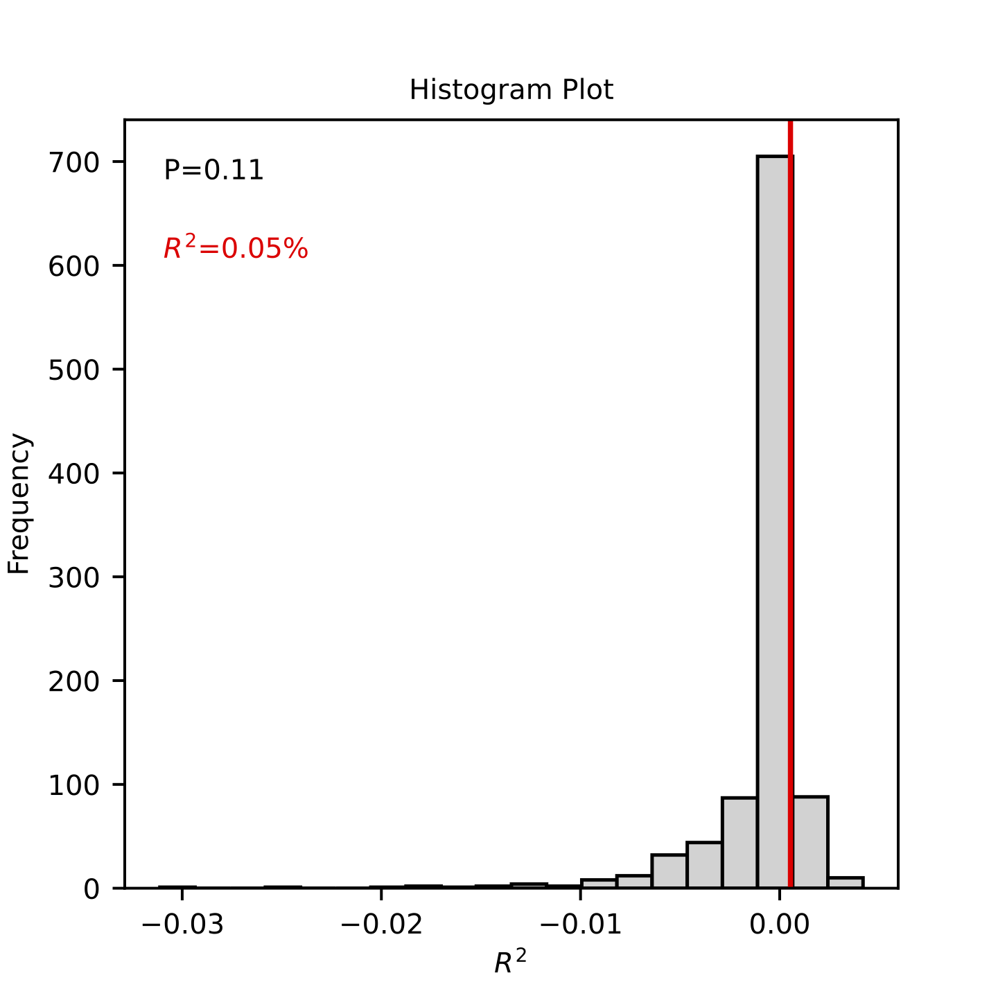
OUTPUT.lasso_histogram_thres_*.pdf: Histogram plot for the observed predictive R2 and random distribution. The random distribution is obtained from samples with a randomly shuffled phenotype. The x axis refers to the observed R2 and the y axis refers to the frequency of R2 s.
OUTPUT.lasso_coef_thres_*.txt:
Example run:
Now run the below command. The below command calculates risk scores for noncoding domain categories.
The de_novo_variants.lasso_coef_thres_3.txt looks like below. This output file lists the categories chosen as predictors for the phenotype through the Lasso regression model.
-c, –corr_mat: Category correlation matrix file. This is the output file from correlation. The file name must have pattern *correlation_matrix*.zarr.
-P, –permut_test: Permutation test file. This is the output file from burden test. The file name must have pattern *permutation_test*.txt.gz.
-c_count, –cat_count: Path of the categories counts file from burden test.
-o_dir, –output_directory: Path to the directory where the output files will be saved. By default, outputs will be saved at $CWAS_WORKSPACE.
–leiden: Perform Leiden clustering. Specify the input matrix type: eigen_vector or corr_mat. By default, None.
-res, –resolution: Resolution for Leiden clustering. By default, 1.
-r, –range: Range (i.e., (start,end)) to find optimal K for k-means clustering. It must contain two integers that are comma-separated. The first integer refers to the start number and must be above 1. The second integer refers to the end. By default, 2,100.
-k, –k_val: K for K-means clustering. With this argument, users can determine K manually. -r and -k arguments are mutually exclusive. If -k is given, -r will be ignored.
-s, –seed: Seed value for t-SNE. Same seed will generate same results for the same inputs. By default, 42.
-T, –tsen_method: Gradient calculation algorithm for t-SNE, which is used in TSNE of sklearn. If the dataset is large, ‘barnes_hut’ is recommended. By default, exact.
-t, –tag: Tag used for the name of the output files. By default, None.
-l, –lambda: Lambda value for parameter tuning. By default, 5.25.
-C, –count_threshold: The threshold of variant (or sample) counts. The least amount of variants a category should have. By default, 20.
-R, –corr_threshold: The threshold of correlation values between clusters. Computed by the mean value of correlation values of categories within a cluster. By default, 0.12.
-S, –size_threshold: The threshold of the number of categories per cluster. The least amount of categories a cluster should have. By default, 2.
–no-parsimonious: Disable parsimonious K selection. By default, the smallest K within the top 5% silhouette plateau is selected. This flag reverts to picking the absolute silhouette maximum.
-p, –num_proc: Number of worker processes that will be used for the DAWN analysis. By default, 1.
The specific descriptions of the output files are as below. Each output file containing a specific pattern (i.e., ) in the file name as below will be found in the output directory. If users set tag, the tag will be inserted in the file name like this: OUTPUT.eig_vecs.tag.txt.gz.